Speech Recognition and Graph Transformer Network II
🎙️ Awni HannunInference Time
The inference of a transcription from a given audio signal can be formulated using 2 distributions:
- The acoustic model (audio to transcription), represented as $P(\mY \mid \mX)$
- The language model, $P(\mY)$
The final inference is obtained by taking sum of the log probabilities of the above two, i.e.
\[\vect{\mY*} = \underset{\mY}{\operatorname{argmax}} \log P(\mY \mid \mX) + \log P(\mY)\]We use the additional term to ensure the transcription is consistent with the rules of the language. Else we may get grammatically wrong transcription.
Beam Search
While returning an output sequence, we can follow the greedy approach, where we take the maximum value of $P(\vy_{t} \mid \vy_{t-1}…\vy_{1})$
However, we can end up missing out a good sequence, which may not have the maximum value of $P(\vy_{t} \mid …)$, as illustrated by the example below.
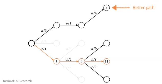
Figure 1: Greedy Approach : Less Optimal Solution
To remedy this, we employ beam search. Essentially, we consider maximum $k$ tokens in terms of probability at each step $t$ of the sequence. For each of these n-grams, we proceed further and find out the maximum.
The illustration below shows how Beam Search can lead to a better sequence.
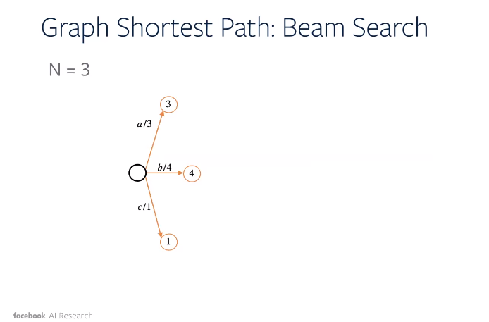
Figure 2: Beam Search : Stage 1
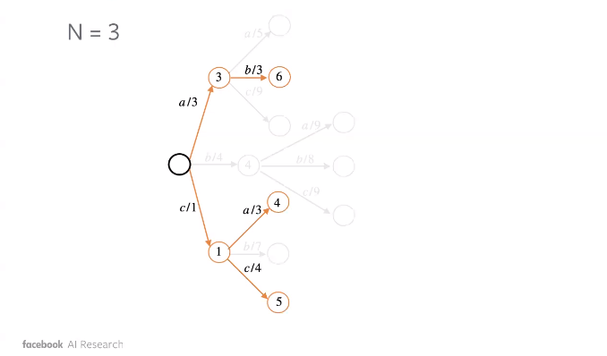
Figure 3: Beam Search : Stage 2
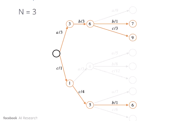
Figure 4: Beam Search : Stage 3
Graph Transformer Networks
We have previously seen Weighted Finite State Automata (WFSA) being used to represent the alignment graphs, as shown before.
Graph Transformer Networks (GTNs) are basically WSFA with automatic differentiation.
Lets look at key differences between Neural Networks (NNs) and GTNs
| NN | GTN | |
|---|---|---|
| Core Data Structure | Tensor | Graph/WFSA |
| Matrix Multiplication | Compose | |
| Core Operations | Reduction operations (Sum, Product) | Shortest Distance (Viterbi,Forward) |
| Negate, Add, Subtract, … | Closure, Union, Concatenate, … |
Why Differentiable WSFAs?
- Encode Priors: easy to encode priors into a graph
- End-to-end: Bridge the training and test process
- Facilitate research: When we separate the data from the code it makes it easier to explore different ideas. In our case graph is the data and the code is operations allows us to explore different ideas by changing the graph.
Sequence Criteria with WFSAs
It turns out that lots of the sequence criteria like connection temporal classification (CTC) can be specified as the difference between two forward scores.
- Graphs A: function of input \mX (speech) and target “output” \mY (transcription).
- Graph Z: function of input \mX, which servers as normalization.
- Loss: $\log P(\mY \mid \mX) = \text{forwardScore}(A_{\mX,\mY}) - \text{forwardScore}(Z_{\mX})$
Other common loss functions in ASR:
- Automatic Segmentations Criterion (ASG)
- Connectionist TEmporal Classification (CTC)
- Lattice Free MMI (LF-MMI)
Lines of code for CTC: Custom vs GTN
| GTN | |
|---|---|
| Warp-CTC | 9,742 |
| wav2letter | 2,859 |
| PyTorch | 1,161 |
| GTN | 30* |
*Same graph code works for decoding.
Different Types of WFS
Weighted Finite-State Acceptor (WFSA)
The bold circle is the starting state and the accepting state is the one with concentric circles.
Example
A simple WFSA which recognizes aa or ab
- The score of aa is 0 + 2 = 2
- The score of ba is 1 + 2 = 3
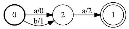
Figure 5: Three Nodes Weighted Finite-State Acceptor (WFSA)
Weighted Finite-State Transducer (WFST)
These graphs are called transducers because they map input sequences to output sequences.
Example
A simple WFST that recognizes ab to xz and bb to yz.
- The score of ab $\to$ xz is 1.1 + 3.3 = 4.4
- The score of bb $\to$ yz is 2.0 + 3.3 = 5.3
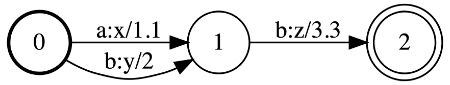
Figure 6: Three Nodes Weighted Finite-State Transducer (WFST)
More WFSAs and WFSTs
- Cycles and self-loops are allowed
- Multiple start and accept nodes are allowed
- $\epsilon$ “nothing” transitions are allowed in WFSAs and WFSTs.
Operations:
Unions
The union accepts a sequence if it is accepted by any of the input graphs.
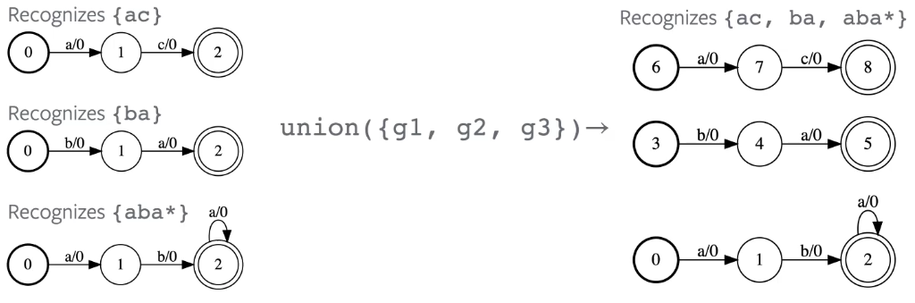
Figure 7: Union Operation Between Three Graphs
Kleene Closure
Accepts any accepted sequence by input graph repeated 0 or more times.
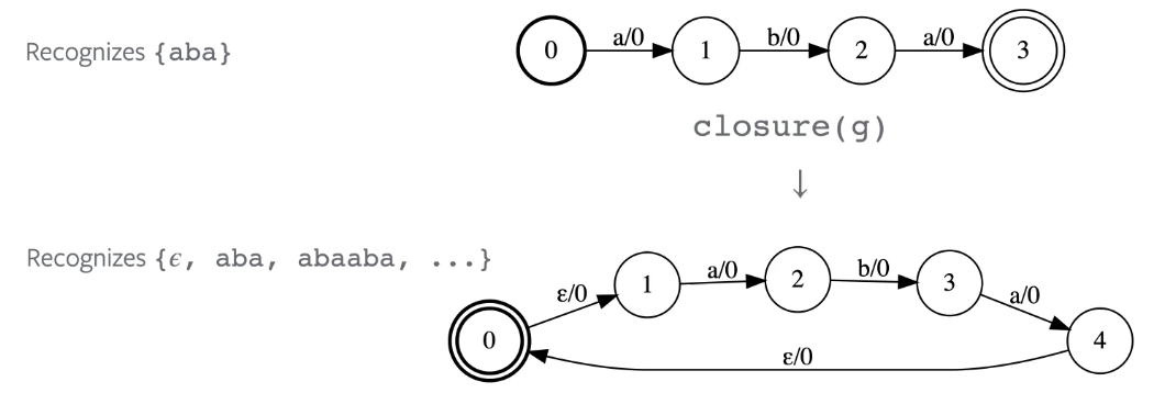
Figure 8: Kleene Closure Operation
Intersect
Similar to matrix multiplication or convolution. This operation is probably the most important in GTNs.
- Any path that is accepted by both WFSAs is accepted by the product of the intersection.
- The score of the intersected path is the sum of the scores of the paths in the input graphs.
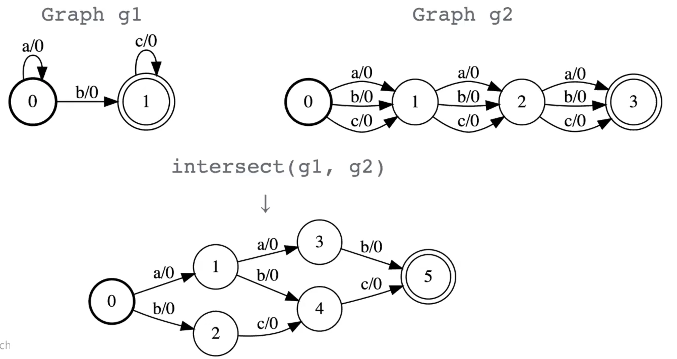
Figure 9: Intersection Operation Between Two Graphs
Compose
It is basically the same thing as intersection but for transducers instead of acceptors.
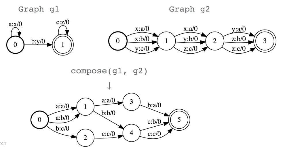
Figure 10: Compose Operation Between Two Graphs
The main thing about composition is that it let’s map from different domains. For example, if we have a graph that maps from letters to words and another graph that maps from words to sentences. When we compose these two graphs we will map from letters to sentences.
Forward Score
Assumes the graph is DAG and an efficient dynamic programming algorithm.
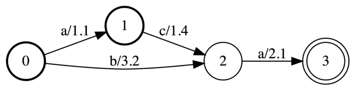
Figure 11: Forward Score is the Softmax of the Paths
The graphs accepts three paths:
- aca with score = 1.1 + 1.4 + 2.1
- ba with score = 3.2 + 2.1
- ca with score 1.4 + 2.1
ForwardScore(g) is the actual-softmax of the paths.
Sequence Criteria with WFSTs
Target graph Y:
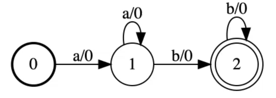
Figure 12: Target Graph \mY
Emissions graph E:
Think of it between two nodes we have logits.
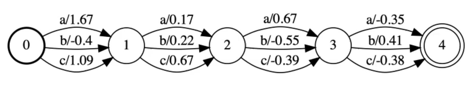
Figure 13: Emission Graph E
Target contrained graph A by intersection(Y, E):
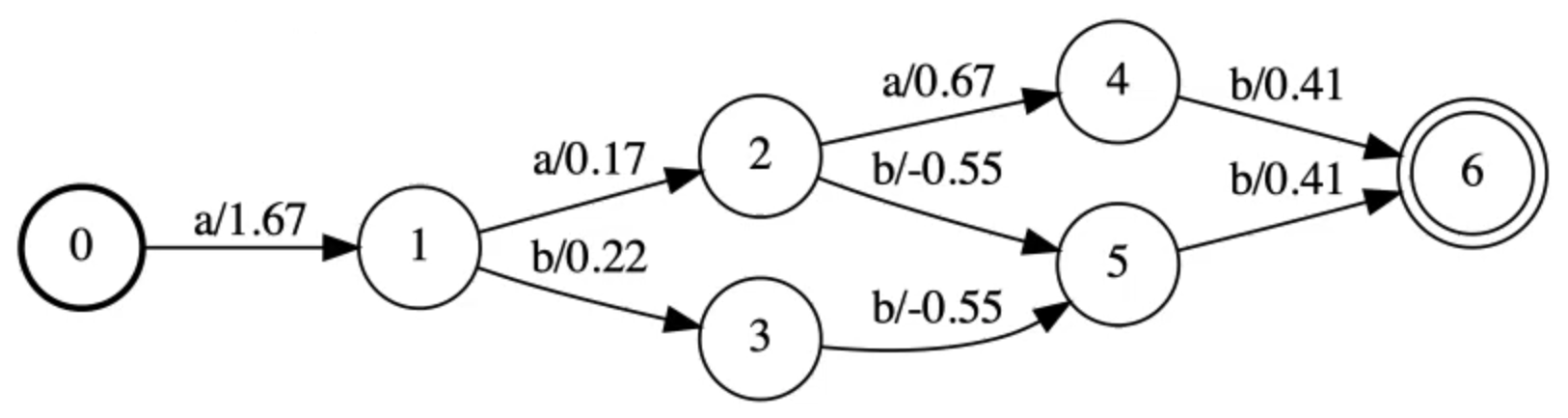
Figure 14: Target Constrained Graph
Loss
\[\ell = - (\text{forwardScore}(A) - \text{forwardScore}(E))\]This is not CTC but approaches CTC.
Code examples:
Make the target graph
Similar to figure 8.
import gtn

# Make the graph
target = gtn.Graph(calc_grad=False)
# Add nodes:
target.add_node(start=True)
target.add_node()
target.add_node(accept=True)
# Add arcs:
target.add_arc(src_node=0, dst_node=1, label=0)
target.add_arc(src_node=1, dst_node=1, label=0)
target.add_arc(src_node=1, dst_node=2, label=1)
target.add_arc(src_node=2, dst_node=2, label=1)
# Draw the graph
label_map = {0: 'a', 1: 'b'}
gtn.draw(target, "target.pdf", label_map)
Make the emissions graph
Similar to figure 9.
import gtn

# Emissions array (logits)
emissions_array = np.random.randn(4, 3)
# Make the graph
emissions = gtn.linear_graph(4, 3, calc_grad=True)
# Set the weights
emissions.set_weights()
ASG in GTN
Steps
- Compute the graphs
- Compute the loss
- Automatic gradients
from gtn import *

def ASG(emissions, target):
    # Step 1
    # Compute constrained and normalization graphs:
    A = intersect(target, emissions)
    Z = emissions

    # Step 2:
    # Forward both.graphs:
    A_score = forward(A)
    Z_score = forward(Z)

    # Compute loss:
    loss = negate(subtract(A_score, Z_score))

    # Step 3:
    # Clear previous gradients:
    emissions.zero_grad()

    # Compute gradients:
    backward(loss, retain_graph=False)
    return loss.item(), emissions.grad()
CTC in GTN
from gtn import *

def CTC(emissions, "target"):
    ...
The only difference is the target which makes it very easy to try different algorithms and the GTN framework is supposed to be similar to PyTorch with different data structure and operations.
Further readings:
- CTC
- GTN
- Modern GTNs
📝 Gyanesh Gupta, Abed Qaddoumi
14th April 2021