SN graphic capabilities
In this article we showcase a few graphic and interactive capabilities of SN — Yann & Léon’s Simulateur de Neurones — called SN Tools, which were vastly ahead of its time. Only when tools are built by their intended users they are truly designed with the needs and nuances of those users in mind, leading to more intuitive, functional, and innovative outcomes.
I assume you’ve read Running SN on Apple silicon and set up your environment, such that executing lush in the command line returns something like:
LUSH Lisp Universal Shell (compiled on Aug  6 2024)
   Copyright (C) 2002 Leon Bottou, Yann LeCun, AT&T, NECI.
SN Tools (docs)
The Netenv library is mainly used for simulating multilayer networks. Indeed, SN 2.8 contains efficient heuristics for training large multilayer networks using several variants of the back-propagation algorithm. This task is made even easier by two dedicated graphical interfaces, NetTool and BPTool.
- NetTool is a graphical network editor. Using NetTool you can build a network using all the connection patterns defined in the library
connect.sn. The program then generates lisp functions for creating and drawing the network.- BPTool is a graphical interface for controlling the training process. BPTool allows you to perform the most common actions allowed by the library
netenv.sn. It provides sensible default values for all the convergence parameters.- A few other tools StatTool, NormTool and ImageTool are useful for browsing and preprocessing the data. These tools are briefly discussed in the last chapter.
The paragraph above comes directly from the manual, which can be accessed by running (helptool) and searched for “introduction to sn tools”.
We’ll start with BPTool, from which menu we can call NetTool.
BPTool demo
Let’s change dir into the backpropagation tool demo folder
cd lush/packages/sn28/examples/bptool
run lush, and load the demo with
(load "load-demo")
A few windows will open, including BPTool.
|
|
|
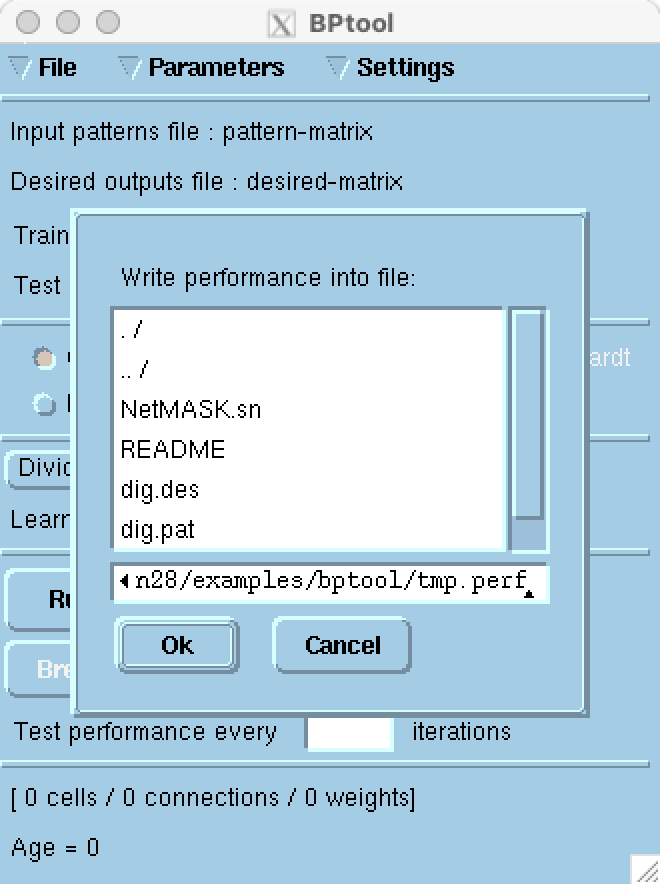
We can discard the request of specifying where to save a performance file by pressing on Cancel.
BPTool is a graphical interface for controlling the training of multilayer networks. […] More precisely, BPTool provides mouse-driven interface to:
- define a network using NetTool,
- load the patterns,
- define a training set and a test set,
- select a training algorithm,
- select the initial weights,
- select the parameters of the training algorithm,
- select the performance criterion,
- train the network,
- measure the performance on both the training set and the test set,
- plot the evolution of these performances during training,
- display the network during training or measurement.
[…]
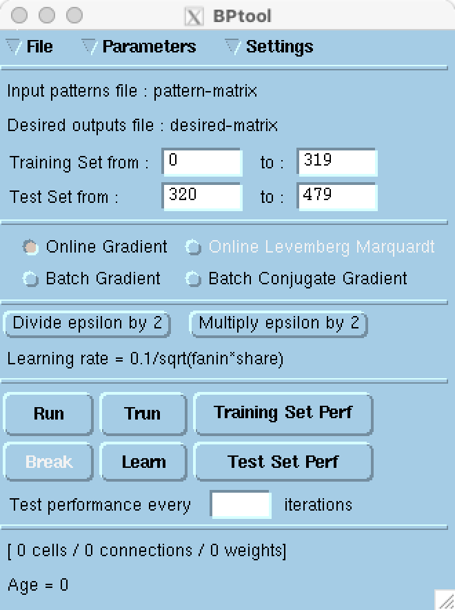
BPTool contains several logical zones.
- The data selection zone lets you select the boundaries of the training and test sets.
- The algorithm selection zone lets you choose a proper training algorithm.
- The learning rates control zone lets you change the learning rates used for the weight updates.
- The training and control zone lets you start and stop the training algorithms.
- The Message zone displays messages such as the age of the current weights and the number of allocated neurons.
Before pressing on Trun, i.e. train & run, we’re going to explore a few menus.
NetTool
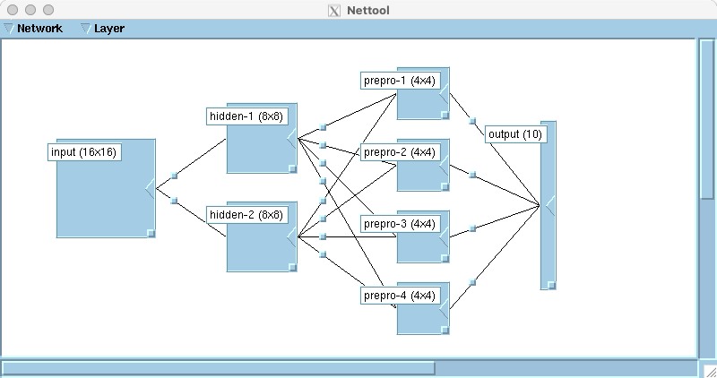
Click on File ▶ Define Network and the NetTool window will pop up.
Here, everything maps to one of the Netenv functions, but with a GUI interface.
You can explore the documentation by executing (helptool) and searching for “overview of nettool”.
There are 4 layers: input, hidden-[1-2], prepro-[1-4], and output. Here, hidden refers to an edge detection stage and preprocessing refers to a feature extraction stage of pattern recognition, which feeds directly the classifier.
Double clicking on each layer’s name allows us to inspect them and change their configuration. The first three layers display mode is set to Gray levels while the output layer uses Hinton, mapping a $\pm 1.2$ range to white/black squares of variable size on a grey background. Moreover, the input has no bias, the hidden and the preprocessing maps have shared bias, and the output layer has full bias.
A layer will stay selected after a single or double click on its label. Therefore, (double) clicking on multiple layers’ label will select them all. To unselect all layers simply click on the empty background.
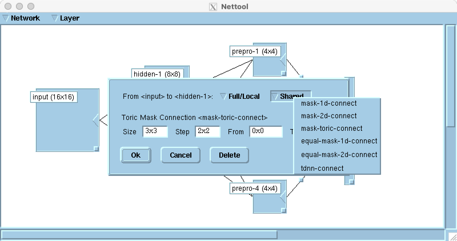
To inspect the model weight typology, let’s click on the square on the wire connecting the maps.
For example the weights from input to hidden-1 use a toric mask connection, which is a circular (toroidal) convolution.
This option can be selected by clicking on Shared ▶ mask-toric-connect.
Moreover, the kernel size is $3 \times 3$, with $2 \times 2$ stride, and the convolution starts from pixel $(0, 0)$ until $(15, 15)$ of the input layer, mapping a $16 \times 16$ feature map to an $8 \times 8$ one.
Clicking on Delete removes the connection from input to hidden-1.
We can recreate the connection by dragging the ◀ of the input map onto the hidden-1 map.
Similarly, a layer can be removed by selecting it (clicking on its label) and choosing Layer ▶ Delete and confirming by pressing Yes. To recreate a layer, select Layer ▶ New and press Ok after having specified the appropriate settings. You can position the map where you want by dragging it, and connect it to the rest of the network by dragging the corresponding ◀’s.
If we would like to use this network at a later time, we can save it as
- a SN file via Network ▶ Save or Create Network and choosing the Save network in file option, or
- a C file via Network ▶ Generate C Function, which can be compiled for a desired target hardware.
For this demo we won’t use this functionality.
Visualising feature maps and output
To be able to visualise the activation of these layers at inference time, one would have clicked on Settings ▶ Display… on the BPTool window, activate the Network checkbox “when Measuring”, and click Apply.
These days the processing is so fast that you would not see much doing so.
Instead, we’re going to define a test pattern tp function, which visualises the model input, internals, and output.
(de tp(n)
   (let ((disp-perf-iteration disp-net))
      (test-pattern n) ) )
Let’s see how the model performs on the first digit of the test set (index 320).
On the Lush interpreter let’s execute
(tp 320)
A Network Window will pop up, showing the output of the convolutions and the final fully connected output.
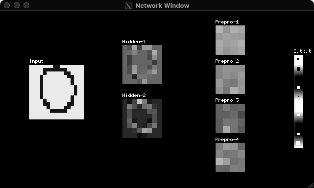
To display the numerical value of the output we can execute
(mapcar nval output)
which for me returns
(-0.0724 -0.2333 0.0079 0.1057 -0.0122 0.1554 0.1172 -0.3977 0.1357 0.292)
The variable output contains the indices of the output units, the nval function return the post non-linearity value of the indexed neuron, and mapcar maps the function nval to each element of the list output, starting from the fist one, i.e. Lisp’s car.
We can explore the rest of Yann’s test hand drawn digits and how the model generates its internal representations and output with a small for-loop.
(for (i tpatt-min tpatt-max) (tp i) (sleep 0.1))
Obviously, since the model has not been trained, the output will not be very insightful. Let’s press Trun on the BPTool panel to train and “run” (evaluate) the model.
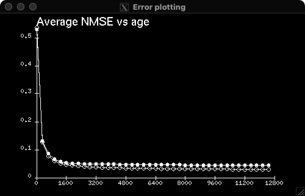
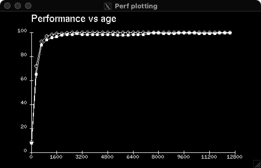
In this case, within 10 epochs, the model performance reaches 100% for both training and testing sets.
|
|
|
You may interrupt learning by pressing Break.
BPTool waits for the end of this learning epoch.
If you press Break twice, BPTool immediately interrupts learning.
If we look at the model outputs with the tp function, we see it has become basically one-hot.
Here is pattern 325 post training and its corresponding output.
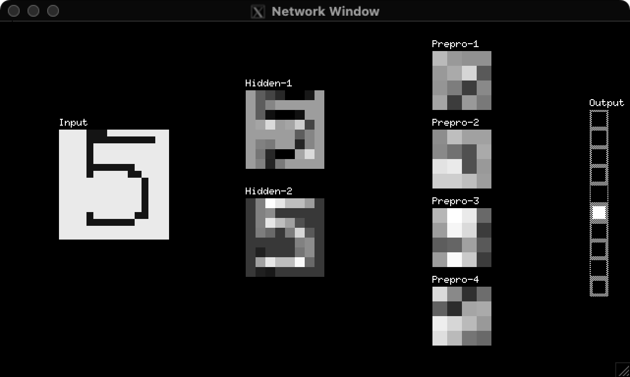
(-0.9508 -1.0668 -0.9659 -0.8942 -1.3663 0.663 -1.0707 -0.8902 -1.2204 -0.7488)
Once again, we can go through all testing patters with the one-liner for-loop.
(for (i tpatt-min tpatt-max) (tp i) (sleep 0.1))
Summary
With the creation of functional custom tools, experimentation becomes more pleasing. The use of graphical user interfaces allows for a separation between programming new functionalities and using different configurations of existent ones. Another apparent difference is the increased discoverability of existing methods, which can be easily tried out in place of the default ones. Finally, a GUI allows the user to readily align their mental model to what is displayed on screen or, conversely, it allows the author to share their mental picture in an unambiguous manner even 40 years in the future, without interacting with the user personally.
More demos
More demos are available in the example folder.
In particular, tsp showcase an approximative solution of the Travelling Salesman Problem using a ring shaped Kohonen map.
How to cite this blog
@misc{canziani2024SN-GUI,
  author = {Canziani, Alfredo and Bottou, Léon},
  title = {{SN graphic capabilities}},
  howpublished = {\url{https://atcold.github.io/2024/09/27/SN-GUI}},
  note = {Accessed: <date>},
  year = {2024}
}