SN: a simulator for connectionist models
This is an English translation of the original French article SN : Un simulateur pour réseaux connexionnistes.
1. Introduction
Writing the core parts of a connectionist network simulation program is often quite simple: the main algorithms often fit in a few lines. However, to effectively use a network, the user must be able to examine the behavior of their network at any moment: this requires writing a significant amount of code to enable this interactivity.
In particular, it is often useful to have graphical outputs or to be able to define a test protocol without having to rewrite large parts of the programs. Furthermore, the very description of the networks is becoming increasingly complex: indeed, most interesting results [7] use complex connection structures, integrating domain knowledge. For example, one might wish to impose local connections, layered hierarchical structures, or constrain certain connections to share the same synaptic coefficient.
Today, there are many network simulation tools: the trend is to develop dedicated languages for simulation or for describing networks [8, 3]. For our own needs, we have written and used for a year a simulator called ‘SN’ (‘Simulateur de Neurones’). In its current version, this simulator allows defining very general network architectures, it implements the back-propagation algorithm and some variants: iterative networks [6], desired state back-propagation [4], second-order back-propagation [5]. This simulator is written in the C language and runs on a number of machines: workstations (SUN, APOLLO), UNIX machines, and vector machines (CONVEX, CRAY).
Sections 2 and 3 describe the main choices made in SN. In sections 4 to 7, we explain the main implemented functions and the elements of the library. Section 8 presents an example of using SN and section 9 discusses ongoing developments.
2. LISP for describing networks and directing the simulation
SN is structured around a language for the description and simulation of networks. Specifically, it involves a small Lisp interpreter. To facilitate portability, this interpreter itself is written in C. Many extensions pertain to the costly operations necessary for connectionist processing, which obviously could not be written in Lisp.
Some simulators are developed around an ad-hoc language, created specifically for network manipulation. In particular, object-oriented languages are often proposed for the ease of hierarchical manipulation of network “objects”: neurons, connections, layers, synaptic weights, etc…
We decided to opt for an existing language. Creating a new language from scratch would have required significantly more time and would have led us to engage in language development activities far removed from the connectionist domain itself. This desire for rapid development guided our choice toward a language that is easy to implement. At this stage, we were hesitating between Lisp and Forth. Although not well-suited for numerical processing, Lisp prevailed, partly because it is universally known, and partly because it allows for easier integration between classical symbolic systems and connectionist systems.
Since this Lisp interpreter is itself written in C, its set of primitives can be easily extended. It suffices to perform a link editing with a C object file containing routines with well-defined arguments.
3. C for calculations
The computation time in a connectionist simulator is determined by:
- Primarily, the operations concerning the connections: calculating the weighted sum of the inputs, error calculation, and weight modification.
- Then, the operations concerning the cells: calculating the states and applying the cell transition function (e.g. a hyperbolic tangent).
- Finally, though less significantly (except for very small networks), the operations performed once during each iteration: accessing the learning patterns, measuring performance, etc…
In SN, all simulation functions concerning connections or cells are written in C, while those concerning the iterations performed are written in Lisp. As a result, the contributions of these different tasks to the overall computation time in SN are not significantly penalized by the relative slowness of Lisp (fig. 1). This slight performance degradation is, in our opinion, more than compensated by the facilities offered by Lisp in describing the network dynamics.
|
Figure 1 – Time allocation comparison between HLM and SN.
|
Comparison of time usage in SN and HLM (a simulator for back-propagation written in Pascal). This involves a back-propagation task on a 3-layer network with 100 fully connected cells. In this example, SN is slightly faster than HLM.
- OP WEIGHTS: weight adjustment.
- OP SUM: calculating the weighted sums for state calculation.
- OP BACKSUM: calculating the weighted sums for gradient calculation.
- CUMUL1: cumulative of the three previous proportions, i.e. the time spent looping on the connections.
- OP CELL: operations related to the cells, mainly the calculation of the sigmoid function.
- CUMUL2: the actual time spent on connectionist calculations. The residual time concerns the operations performed once during each iteration. Only these operations in SN are written in Lisp.
4. Network description
In SN, describing networks is essentially a construction operation. To describe a network means to define a Lisp function, parameterized or not, that builds it.
We have thus defined two types of primitives:
- The first type creates new cells, either one by one or by layers. For the back-propagation algorithm, for example, there is the primitive
newneurons:(setq layer (newneurons 5))This puts a list of five new cells into the variable
layer. - The second type connects the created cells with the previous ones: simple connection, shared weight connection, complete layer-to-layer connection.
A simple connection is defined by the primitiveconnect:(connect a1 a2)This establishes a connection from cell
a1to cella2.
In the current version, all other network description functions are constructed in Lisp from these two classes of functions. Simple networks can thus be built by calling a single function, itself defined in Lisp in the standard library. In particular, the function build-net:
(build-net '((input 400) (hidden 50) (output 76))
           '((input hidden) (hidden output)))
builds a multi-layer network containing 400 cells in an input layer named input, 50 hidden cells in a layer named hidden, and 76 output cells in a layer named output. Additionally, it indicates that the connections are complete from layer to layer.
5. Simulation
Simulation primitives can be classified into four main categories:
- The first category serves to set or examine the states of a group of cells.
- The function
get-pattern:(get-pattern array n layer)allows, in particular, to force the states of a layer of cells with values extracted from the n-th row of an array. It is generally used to impose input states on the network.
- The function
state:(state layer)retrieves the states of the layer in a list.
- The function
- The second category aims to update the states or any other variable of a group of cells based on the states of their neighboring cells.
- For example, the two main functions of the gradient back-propagation algorithm are:
(update-state layer)
(update-gradient layer)
These functions simply calculate the states and error gradients associated with a layer of cells based on the states of upstream cells and the gradient of downstream cells.
- For example, the two main functions of the gradient back-propagation algorithm are:
- The third category applies an algorithm for adapting the synaptic coefficients.
- In the case of back-propagation, the primitive:
(update-weight)modifies the weights according to the back-propagation algorithm, taking into account the states and gradients of the upstream and downstream cells, the current learning rate, momentum, and decay.
- In the case of back-propagation, the primitive:
- The fourth category of functions allows controlling various operating parameters of the network: initial values of synaptic coefficients, type and parameters of transfer functions associated with the cells, learning rate, etc… Each of these parameters can be controlled independently.
Additionally, library Lisp functions implement higher-level concepts: for example, they allow performing learning cycles, measuring performance, and generating graphical outputs. They are also responsible for setting all parameters consistently. See below in the example for the function epsi.
6. Graphics
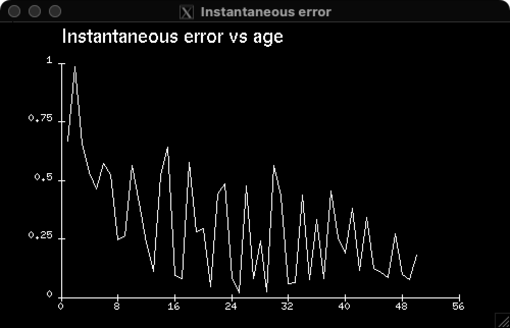
As mentioned earlier, it can be very useful and always very effective to have graphical representations of the network, the error curve, or the magnitudes of network variables (activity states, gradients, weights, etc.).
To this end, SN is equipped with graphic functions. In addition to some of the usual functions of graphical systems available on workstations, such as:
(create-window posx posy sizex sizey name)
(draw-line x1 y1 x2 y2)
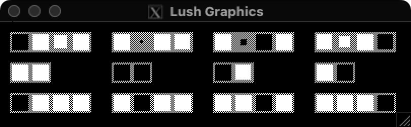
there are also functions specialized in representing analog values. These functions allow drawing the shape of a network with patterns proportional in size to the magnitude of various network variables.
For example:
(draw-list x y real_list ncol pix apart smax)
produces a ‘square’ drawing of the real values contained in the list real_list. By assembling these draw-list functions, one can build visualization functions for entire networks (fig. 2). To usefully complement these functions, we have written a simple curve plotting library in Lisp. It allows drawing axes and plotting curves in real coordinates (fig. 2).
|
|
|
|
|
Figure 2 – Error as a function of time for the 4-2-4 decoder and inference for the four patters (above), performance logs (below).
|
$ grep perf logs.txt
patterns{0-3}, age= 0, error=0.6718, performance=  0
patterns{0-3}, age=10, error=0.2258, performance= 25
patterns{0-3}, age=20, error=0.1810, performance= 50
patterns{0-3}, age=30, error=0.2156, performance= 50
patterns{0-3}, age=40, error=0.1663, performance= 50
patterns{0-3}, age=50, error=0.0748, performance=100
7. Libraries
The existence of a language for network description and simulation allows for the construction of significant libraries. For instance, the standard library associated with the gradient back-propagation alg08-05orithm contains all the high-level definitions needed to direct the simulation in terms of learning cycles, test stages, and performance measurement criteria:
(run 100 20)
allows, for example, to run 20 cycles of 100 learning iterations each, followed by a test stage.
(while (< (perf) 98)
  (learn 200))
requests to perform cycles of 200 learning iterations until the performance on the learning set exceeds 98%. One can envision operations as complex as desired.
These libraries thus contain a substantial part of our knowledge about networks and how to set various parameters. For example, in the case of the gradient back-propagation algorithm, the function:
(SMARTFORGET)
reinitializes the weights to random values within an interval that takes into account the transfer function used and the usual scaling laws, particularly regarding cell connectivity.
8. An example: “the 4.2.4 encoder-decoder”
Here is a small concrete example: “the 4.2.4 encoder-decoder”. We have 4 forms on 4 bits: +---, -+--, --+-, ---+, which we want to encode into 2 bits.
We use a fully connected multilayer network operating in auto-association. Thus, the input and output layers each contain four cells, while the hidden layer contains only two. To correctly associate each of these 4 forms with itself, the network will exhibit a 2-bit encoding of these forms in its hidden layer. For this purpose, gradient back-propagation learning is used.
This problem, from a strictly mathematical point of view, is in fact just Principal Component Analysis (PCA). Its main interest here is to show how SN works and can be used.
Here is an example of an SN program, running in the standard environment, to solve this problem:
; Allocate memory for 40 cells and 1000 connections.
(ALLOC-NET 40 1000)

; Create a three-layer network, fully connected
; with sizes 4, 2, and 4.
(build-net '((input 4) (hidden 2) (output 4))
           '((input hidden) (hidden output)))

; Create an array containing the patterns
; The symbols pattern-array and desired-array are those used
; by the standard library.
(dim pattern-array 4 4)
(for (i 0 3)
  (for (j 0 3)
    (pattern-array i j (read) ) ) )
       1 -1 -1 -1
      -1  1 -1 -1
      -1 -1  1 -1
      -1 -1 -1  1

; Working in auto-association.
(setq desired-array pattern-array)

; Specify the patterns to use for learning.
(ensemble 0 3)

; Definition of the transfer function.
; i.e., f(x) = 1.68tanh(2x/3) + 0.05x
(nlf-tanh 0.666 0.05)

; Random initialization of weights
; i.e., in [-2.38/sqrt(Fanin), 2.38/sqrt(Fanin)]
; This corresponds to framing the probability density of
; weighted sums between the points of maximum curvature
; of the transfer function.
(SMARTFORGET)

; Initialization of the learning rate
; For each connection, epsilon is 1.0/Fanin.
(epsi 1.0)

; Display mode during learning
(set-disp-nil) ; silent.

; Measurement criterion: A result is considered correct
; if the quadratic error is less than 0.2
; This criterion is used by the perf function.
(set-class-lms 0.2)

; Learn until a satisfactory rate is achieved.
(while (< (perf) 100)
  (learn 10) )
This learning takes about 10 seconds on an Apollo workstation. By enriching this skeleton with graphical functionalities and using the appropriate display mode, you get the screen whose copy is in figure 2.
9. Planned developments
Several major improvements are currently underway:
-
Rewrite a Faster and More Flexible Lisp Interpreter: This new interpreter should allow easier interfacing of C functions and include nearly everything expected from a non-dedicated Lisp interpreter. Additionally, it will be capable of treating cells or any other abstract objects specific to the connectionist domain as full-fledged Lisp atoms.
-
Modify Simulation Functions: These modifications aim to accommodate several types of cells or connections, each with different behaviors. We hope to be able to simulate hybrid networks and networks working in cooperation.
-
Write C Modules for Major Connectionist Algorithms: These will not only include the gradient back-propagation algorithm but also associative memories, topological map models like those of Kohonen and Grossberg, and the Boltzmann machine.
-
Harmonize All Added Functions: Over time, various functions have been added as we experimented with SN. This harmonization will make the system more cohesive.
This new version is expected to be available by the end of 1988 on workstations (Apollo, Sun).
10. Conclusion
We have developed a general neural network simulation system that, in its current version, allows for:
- Very flexible definition of a network architecture
- Definition of dynamics on this network
- Conducting learning and testing experiments
- Real-time visualization of network operations
This tool has enabled us to undertake applications of various scales: small educational examples, validity tests of new algorithms, and full-scale applications (image and speech recognition). Our experience has convinced us that using such a tool significantly reduces the necessary development time.
This simulator is used in our laboratories as well as in several companies.
11. Bibliography
-
W.A. Hanson & al., “CONE COmputational Network Environment” - in Proceedings of the IEEE First International Conference on Neural Networks, pp 531-538, June 87.
-
D.B. Parker - “Optimal Algorithms for Adaptive Networks: Second Order Back Propagation, Second Order Direct Propagation, and Second Order Hebbian Learning” - in Proceedings of the IEEE First International Conference on Neural Networks, II-593, June 87.
12. How to cite this blog
@misc{canziani2024SN,
  author = {Canziani, Alfredo},
  title = {{SN: a simulator for connectionist models}},
  howpublished = {\url{https://atcold.github.io/2024/08/05/SN}},
  note = {Translation. Accessed: <date>},
  year = {1988/2024}
}